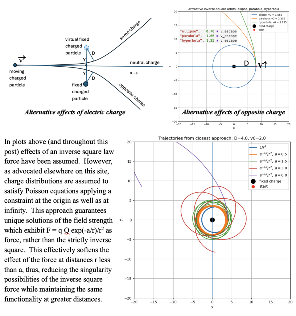
Let’s consider the energetics of a two-object system. Objects have mass and/or charge that distorts their interactive trajectories. If they were completely neutral, then their paths would be unaffected by the position or trajectory of the other. If the relevant effect of their charge was to exclusively repel the other, any initial tendency of approach would be thwarted with a hyperbolic trajectory that ultimately separates objects without limit.
The more interesting of the effects involve attraction for which there are cyclic orbits if relative velocity remains less than the ‘escape velocity’. So, let’s consider that case.
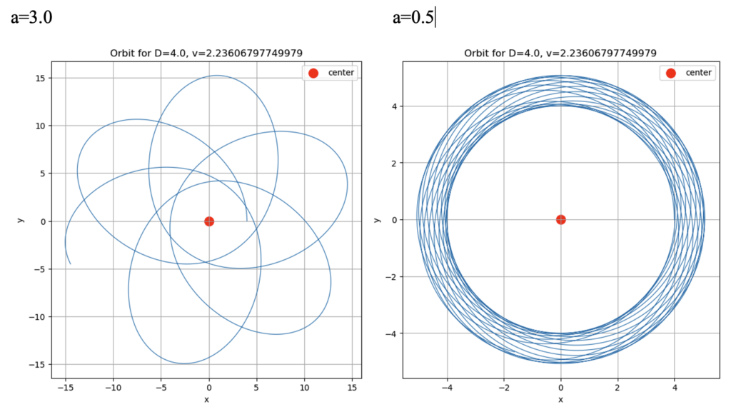
A direct comparison for various tangential velocity values at apogee or perihelion separation distances is shown below. While never approaching closer than the initial separation of the inverse square orbit, these Poisson orbits exhibit precession around the inverse square orbit.
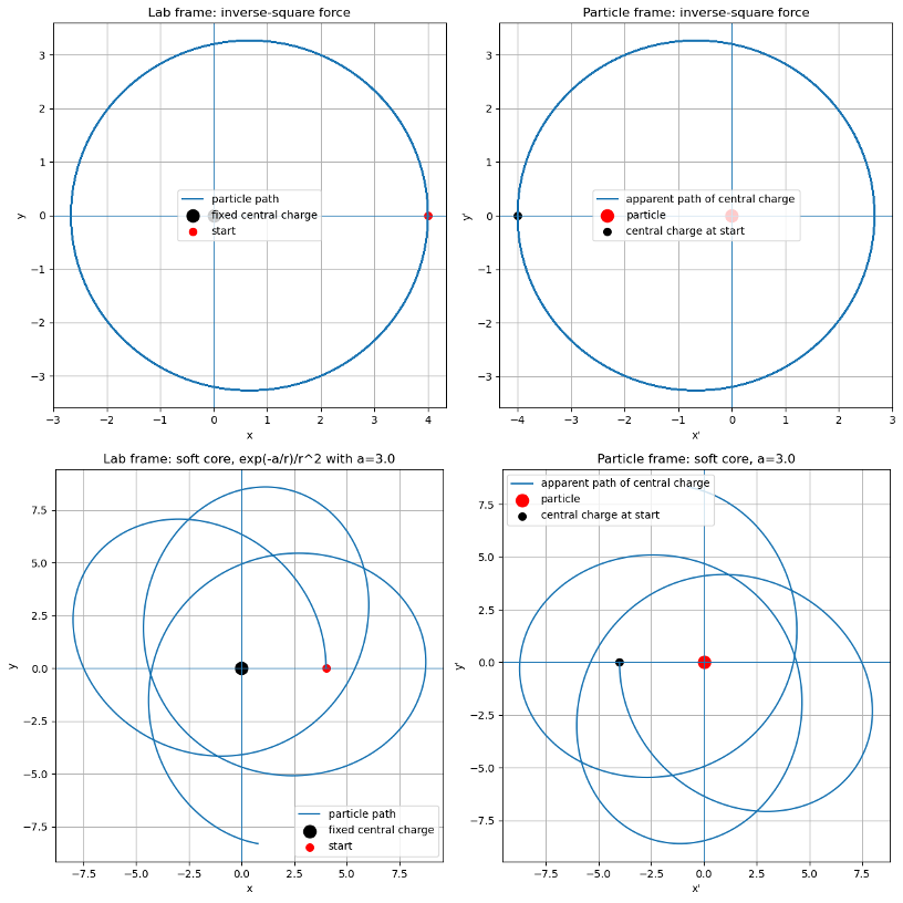
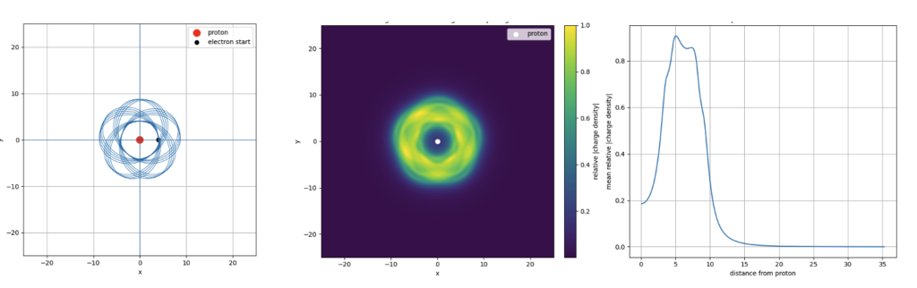
For some perspective, what does the ‘central charge’ path look like from a particle’s perspective?
In the plots for the alternative Poisson force situation, we have calculated the orbits assuming the ‘orbiting’ object is a strictly a ‘point charge. But of course it too must satisfy Poisson boundary values. But when the exponential factor is very small relative to trajectory distances, an inverse square law force is an approximation that is completely justified when 1 >> a/r.
In center of mass laboratory coordinates, orbital motion is primarily that of the less massive of the objects. In an alternative Poisson approach mass is determined by charge as accommodated by calculating a ‘self-energy’ associated with ‘rest mass’ of an associated charge distribution ‘particle’:
m = Q2 / 2 a c2
Thus, the more broadly distributed the charge (larger value of a), the less its mass. The more massive such a Poisson object is, the tinier it will be in the sense of the bulk of its distribution being confined to a much smaller region of space. And since we tend to think of the ‘smaller’ object as orbiting the larger, the reversed perspective illustrated at the right in the preceding figures is perhaps the most accurate to envision but of little other consequence.
For orbiting ‘particles’ that are, in fact, just Poisson charge distributions, the tracing out of their orbits does not indicate the density of an associated charge ‘cloud’ at any given location over any finite interval of time. In the following diagrams the progression of orbits over a given interval of time is shown at the left and the charge cloud density is illustrated at the center, with a plot of the density at the right. The plot suggests that this is probably an ‘non-resonant’ orbit.
As shown in the first triplicate figure above, the tangential initial velocity of the orbits is either at the closest or furthest point on an orbit around a central charge. On perfect inverse square orbits, these points on the elliptical orbit are called the ‘perihelion’ and ‘apogee’, but in these precessing orbits we speak of periapsis and apoapsis instead. With a modified inverse square functionality, we do not in general observe closed orbits, precession may (and much more likely, will) proceed indefinitely. However, with certain combinations of initial separation and velocity, the initial (or just a previous periapsis or apoapsis) will be reached, in which case a rosette pattern is complete. When the orbit lines up with itself in this way, we call it ‘resonance’.
Each time the orbiting object reaches periapsis, the precession angle about the center at which it is achieved will advance by some incremental angular amount:

Where p is the number of turns the orbit has taken around the central charge and q is the number of cycles the orbit has made. If both p and q are integers, i.e., the ratio is rational, the orbit will be closed. For a strict inverse square law, p/q = 1.0. But this condition is very dependent on the structural parameters D and v0 for the alternative Poisson orbits. For a given D and v0 plot the orbit numerically around to the next periapsis to determine Dq/2p from which to obtain p/q. Do this again for the dame D through the range of velocities v0. Then repeat for a set of D values.
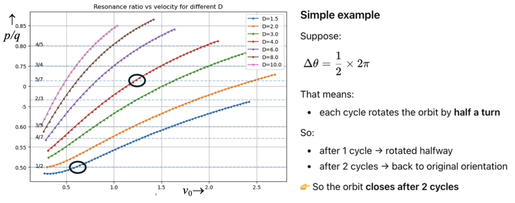
But there are only certain combinations of initial separation and velocity (energy) for which a resonance can be found as shown at left above. Below are two plots of resonances that apply.
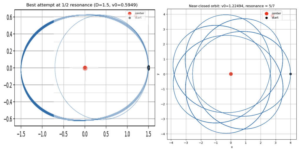
The inverse square law analogy cannot be viably compared since at that low velocity and short distance of the p/q = ½ resonance, because in the inverse square ‘orbit’ the particle collapses into the central charge. By increasing the velocity by a factor of six from 0.5949 to 2.9212 we get a somewhat similar inverse square orbit shown faintly in the left diagram. The completed rosette for the p/q = 5/7 resonance is shown at the right.
But let’s look at these resonance ratios in a little more detail. Here we illustrate the functionality of these curves for values of D from 0.05 to 30. The exponential factor a=3.0 in all these plots and the ones above.
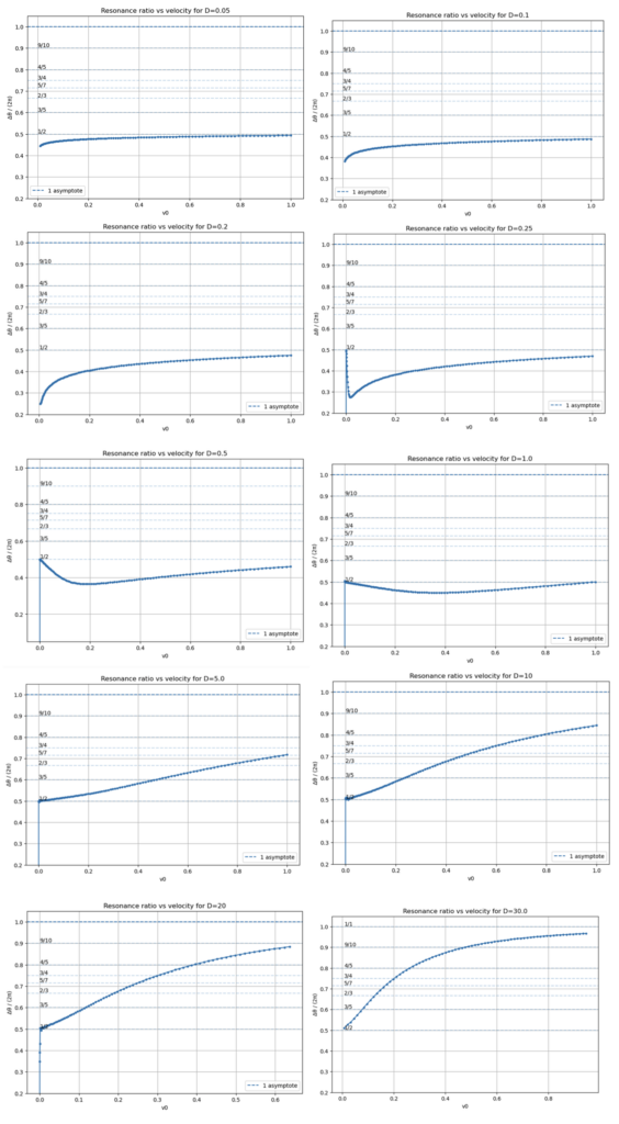
What is particularly interesting here is the behavior of the curves for which D < 1.0 where 3 D < a. In particular, for D=0.5 we have:
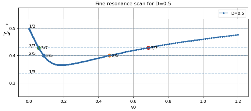
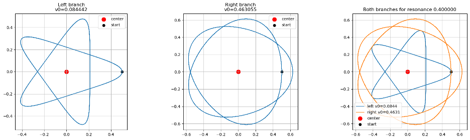
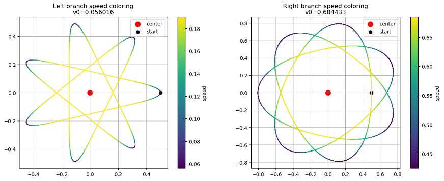
There are two values of v0 for the same resonances. Let’s look at the two orbits associated with the dual resonances:
First we look at the 2/5 resonance:
Then the 3/7 resonance:
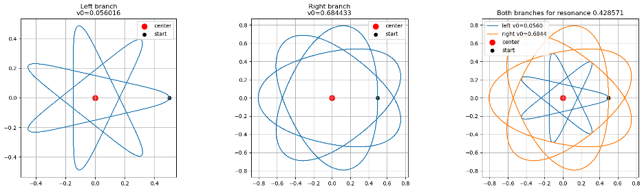
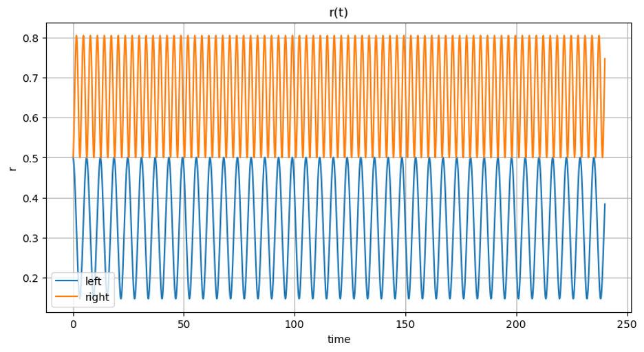
The two orbits in both cases have exactly the same initial velocity and distance from the center, yet there are two orbits, one fully contained within the other. The velocity profiles through the two different orbits for the 3/7 resonance are shown below:
They would not both return to the same periapsis at the same time. Their periods are different as shown below:
That’s enough for now. More later.
Leave a Reply